
Geoida
Help
|
|
Geoida |
|
This topic deals with the statistical options that may be set for least-squares adjustments and how those settings are used to affect the analysis of the results of adjustment.
Statistical Options
Global statistical and analysis settings for least-squares adjustments are made in the Definitions menu Preferences option:
.PNG)
|
The initial settings accessed here are applied as defaults to
all jobs in any normal Survey menu traverse-reduction
options or the Least Squares Network Adjustment option.
Further modification to these default settings to suit the
individual data sets being processed, may be made within the
various data processing options by clicking the  button on each form.
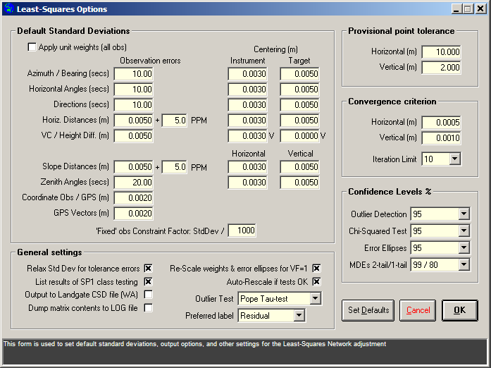
Both the global settings and the local option settings for least squares adjustments are made within the Least-Squares Options dialog window:
|
|
More Info: |
When Geoida is running, details of the purpose and use of each control in this window will be displayed in the bottom panel when the mouse is passed over any active object. |
Provisional point tolerance
The values for horizontal and vertical provisional point tolerance are specified in the Least-Squares Options window, accessed via the LS Options button, and is used for checking entered observations for input errors - the standard value is 10 metres horizontal and 2 metres vertical. A warning message is given if an observation to a particular point places the computed point more than this tolerance value away from the point's provisional coordinate value or if the difference between the observed and calculated angle or distance observation is greater than the tolerance, and the observation is marked with 'XX' in the adjustment report. The computation continues if the user agrees. The purpose is to indicate observations or provisional coordinates that either may be in error or were entered incorrectly. The treatment in such cases would be to (i) check the observation data, (ii) determine a more accurate estimation of the point's true coordinates, or (iii) relax the provisional point tolerance value. Check the log file (jobname.LOG) to see details of the observations and points affected.
Relax SD on Entry Errors
The option Relax Std Dev for tolerance errors (LS Options button in Least Squares Network Adjustment or Least Squares Adjustment Options button in Preferences) helps locate gross errors and blunders. If isolated observations appear to be grossly in error, the standard deviations may be relaxed (enlarged by a set amount - 1000 times) for easier detection of blunders or entry errors. Much of the adjustment will thus be thrown into a bad observation such that its final adjusted value should be close to its correct value, while other surrounding reliable observations will suffer little distortion. Cross this box to perform this function. Observations affected by tolerance errors will be marked in the summary by XX - a single observation thus marked would suggest that the observation itself may be in error, while several observations in a cluster marked in this way might indicate that a provisional point location may be in error.
Centerings and A-Priori Standard Deviations
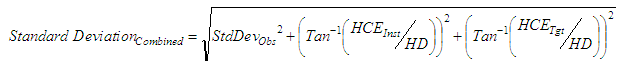
Centring errors are combined with observation errors to derive
the a-priori standard deviations used in the adjustment. The
following formulae are applied for the different observation
types:
Azimuths, Directions
|
Horizontal Angles

|
Horizontal Distances
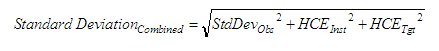
|
Vertical (Zenith) Angles

|
Height Differences

|
| where: | StdDevObs | = | Standard deviation of the observation measurement |
| HCE | = | Horizontal centring error | |
| VCE | = | Vertical centring error | |
| HD | = | Horizontal distance | |
| SD | = | Slope distance | |
| VD | = | Vertical distance |
Convergence criteria
Iterations of the least-squares network adjustment stop when the amount of adjustment made to all points is less than the convergence criteria as specified by the Convergence criterion - Horizontal or Vertical settings in the Least-Squares Options window, accessed via the LS Options button. If the adjustment does not converge after the pre-set number of iterations (10), the software will prompt for another 10 iterations if the user so requires and will continue to do so until the user stops the process. Obviously there is no point in continuing to iterate indefinitely - if the adjustment has not converged after the first 10 or so iterations then the data, standard deviations, convergence criteria, etc need to be re-assessed, or there is a serious error in the network, for example, a major observational blunder, incorrect point numbers specified, etc.
Outlier tests and data snooping
Standardised Residuals enable the direct comparison of the precision of the various observation types by reducing the residuals from different observation types to a common level. This is achieved by simply scaling each adjusted observation's residual by either (depending on the test) its assigned a-priori standard deviation or a-posteriori standard deviation, i.e. it is the ratio of the observation's residual divided by its particular standard deviation.

|
Thus a simple test for outliers sometimes used is that for an observation whose standardised residual is more than 3 times greater than the standard deviation of unit weight (3-sigma level, or 99.7% confidence level), either:
Four tests involving standardised residuals for detection of gross errors are available in Geoida: Baarda’s W-test, Pope’s Tau-test, the Tau-Max test, and the Standardised Residual Test. The preferred test may be defined in Least-Squares Options from the Outlier Test drop-down selection list; the confidence level for the test is defined in the Outlier Detection list.
Baarda’s W-test - Baarda's 'data-snooping' technique
assumes that the a-priori observation variances are reliably known
such that the computed a-posteriori variances should be compatible
with the a-priori values, i.e. that the null hypothesis applies,
where the a-posteriori variance factor of the adjustment is
statistically equal to 1.00. Failure of the test may be because of
incorrect estimation of a-priori variances or weighting, or because
gross errors exist within the observation data. The test fails if
the residual's magnitude is greater than the test statistic for the
given confidence level, times the a-posteriori standard deviation
of the observation. I.e., for the i th
observation,
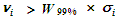
|
Note that this test may be misleading and unreliable if the computed variance factor of the adjustment is not statistically equivalent to 1.0 (as determined by the Chi-squared test) because the test assumes that the observation a-priori standard deviations are known (i.e. correct), thus if the Chi Squared test FAILS then the a-priori estimations were NOT correct and the outlier test cannot be used.
Pope’s Tau-test - The Pope Tau-test assumes that the
observation a-priori standard deviations are not adequately known
or are considered unreliable. The test is applied to each
observation's a-posteriori standardised residual derived from the
variance-covariance matrix of the residuals. The test statistic is
derived by assuming that the null hypothesis follows the
tau-distribution as degrees of freedom increases; an outlier is
indicated where the standardised residual exceeds the test
statistic.
The test assumes that only ONE observation is in error, hence only the observation having the largest outlier test value should be discarded, followed by a re-adjustment of the network. This process is repeated until all anomalies have been eliminated. Due to the nature of the test, it is always possible that some gross errors may remain undetected, especially if they are small.
Refer to other sources for further details of the Pope Tau-test, eg Concepts of Network and Deformation Analysis (W F Caspary, 1988) or Geodetic Network Analysis and Optimal Design: Concepts and Applications (S Kuang, 1996).
Tau-Max test - The Tau-Max test improves Pope's Tau
test by reducing the significance level by the inverse factor 2n
(twice the number of observations) and computing a new Tau value
accordingly. Hence the Tau-Max test is a much more conservative
test than Pope's Tau test because it considers also the number of
observations contained in the set and is less likely to reject the
original hypothesis. The test assumes that only ONE observation
will be in error, hence only the observation with the largest
outlier should be removed before re-adjusting the network and
re-testing.
Refer to other sources for further details of the Tau-Max test, eg Concepts of Network and Deformation Analysis (W F Caspary, 1988) or Geodetic Network Analysis and Optimal Design: Concepts and Applications (S Kuang, 1996).
A-Priori Standardised Residual Test - This is a
simple but commonly used test where the test statistic is the value
of an observation’s standardised residual (the ratio of its
residual to its own a-priori standard deviation) and is
compared against the selected confidence level factor - if the
confidence level is exceeded (i.e. the residual is larger than the
confidence-level factor times the standard deviation) the
observation is flagged as a possible outlier.
This test is valid when the a-posteriori Variance Factor or Standard Deviation of Unit Weight of the adjustment is statistically equal to 1.00 (Chi-Squared test passes) which confirms the a-priori standard deviations of the observations as realistic. However the test may be misleading and lead to unreliable conclusions if the variance factor is NOT 1.0 whence it should be treated with caution. In this latter case the network should be first readjusted by scaling the a-priori weights to achieve a variance factor of 1 - any observations now failing the test may justifiably require attention.
Test Results - Any observation whose residual fails
the test, is marked 'Failed' to indicate that the
observation may be marginally or grossly in error. However, the
reason that an observation is in error may not be obvious since the
magnitude of the error may be relatively small. Marked observations
should be examined carefully, bearing in mind that an observation
marked as being in error may actually be influenced by one or more
other observations adjacent to it. If a suspect observation is
deemed to be correct so far as it is possible to determine, it may
be necessary to either relax its a-priori standard deviation or
remove it from the adjustment to reduce the strain on the network.
Refer also to Relax SD on Entry
Errors above - while most observation outliers will not
fall into the category of 'entry error' blunders, turning on the
Relax Std Dev for tolerance errors option may occasionally
assist in isolating suspect observations or elimating those that
were marked as having failed the outlier test (due to the influence
of adjacent poor observations) but are still actually valid.
If the network includes isolated points coordinated with no redundant observations (eg radiations), these may cause the residuals test to fail because the residual variances are zero, even though the presence of the radiation observations has no other adverse effect upon the adjusted points. If processing from Extract file, the radiation observations could be commented-out and the network adjustment re-run without any change to the adjustment except to achieve a satisfactory report.
Confidence Region Scalars
Required Confidence Level % |
Multiplying Factor | ||
| 1D Standard Deviation of Error Bar or Observation |
2D Standard Error Ellipse |
3D Standard Error Ellipsoid |
|
| 20.0 | - | - | 1.00 |
| 39.0 | - | 1.00 | 1.36 |
| 50.0 | - | 1.18 | 1.54 |
| 68.3 | 1.00 | 1.52 | 1.88 |
| 90.0 | 1.65 | 2.15 | 2.50 |
| 95.0 | 1.96 | 2.45 | 2.79 |
| 99.0 | 2.58 | 3.04 | 3.37 |
| 99.5 | 2.81 | 3.26 | 3.58 |
| 99.7 | 3.00 | ||
| 99.9 | 3.29 | ||
Global chi-squared unit variance test
The value of the a-posteriori unit variance should approach the hypothetical a-priori assumed value of 1. If it is significantly different from 1, the a-priori standard deviations of the observations should be modified such that
Additionally, the standard deviations of individual observations may be modified.
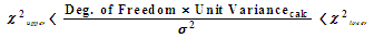
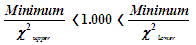
The a-posteriori unit variance is subjected to the chi-squared test whence the upper and lower limits for the chi-squared distribution for the current degrees of freedom are applied to the current unit variance to test against unity as follows …
|
Transposing for  …
…

|
|
The test passes if the value 1.000 falls within of the range calculated. The values for the chi-squared test printed in the summary are the range for the a-posteriori variance factor for the current adjustment as derived from the chi-squared range for a variance factor of 1.000 for the current degrees of freedom. The result of the test is indicated in the summary.
If the test fails, the computed a-posteriori variance factor is incompatible with the null hypothesis a-priori variance factor of 1.000. In this case, if the residuals of the observations are sufficiently small compared to the accuracy of the instruments used to achieve the observed measurements, and provided that no observation failed the test for outliers (see Outlier test and data snooping above), then the adjustment statistics may be recomputed with the weight matrix scaled by the amount of the computed variance factor, to achieve a final a-posteriori variance factor of 1.000. The user is prompted with the following message (eg) …
| The first estimate of the a-posteriori Variance Factor is
0.462 which fails the Chi-squared global test at the LOWER end. However, no residual outliers have been detected and if the magnitude of the residuals (corrections) is relatively small, it is accepted practice to scale the weights by the amount of the computed variance factor and recompute the adjustment. Do you wish to re-compute to achieve a variance factor of 1.00? |
If the user responds with 'Yes', the weight matrix is multiplied by the inverse of the computed variance factor and the statistics are recomputed. The new variance factor computed should now be 1.000 and the chi-squared test will pass provided that there are no new outliers detected.
However, if residual outliers DO occur, the Chi-squared test will still fail but the prompt shown above will now display (eg) …
| The first estimate of the a-posteriori Variance Factor is
7.935 which fails the Chi-squared global test at the UPPER end. Residual outliers DETECTED !! It is NOT the usual practise to re-scale the weights by the amount of the computed variance factor and re-compute the adjustment, but ... Do you wish to re-compute to achieve a variance factor of 1.00? |
In this case the user may still respond with 'Yes' to rescale for a new variance factor of 1.000 as previously, allowably if the variance factor is close to the range required, but with due caution in the acceptance of the results of the adjustment.
Ideally, if the Chi-squared test fails, a process of trial and error should be followed in which the observation standard deviations are repeatedly reassessed and manually modified followed by re-adjustment until the test passes, rather than simply re-scaling in response to the above prompts, and particularly so if the a-posteriori variance factor is significantly not close to 1. However, if the test does not pass but error ellipses are scaled by the a-posteriori sample standard deviation according to the Scale error ellipses by sample Standard Deviation setting in the Least-Squares Options window, then the size of the error ellipses and consequently the results of SP1 class testing (if used) should be consistent with those obtained after re-scaling of the weight matrix and re-computing in response to the above prompt.
If the Chi-squared test passes in the first instance, the standard deviations of point locations and their error ellipses have been effectively scaled by the amount of the a-priori standard deviation of 1.000, i.e. they are not scaled because the adjustment is statistically sound. However, scaling the standard deviations and error ellipses by the amount of the a-posteriori sample standard deviation after a failed Chi-squared test, has an effect similar to then scaling that weight matrix by the a-posteriori variance factor to derive standard deviations and error ellipses of the adjusted point locations, and the summary shows the scaled a-priori standard deviations as should have been used to achieve a variance factor of 1.000 without re-scaling.
Scaling of Error Ellipses
Refer to the section Global chi-squared unit variance
test above for discussion of the need for variance factor or
error ellipse scaling.
When should scaling be applied?
Scaling of the error ellipses can be achieved in 1 of 2
ways:
Using either of these methods has the same effect - Geoida uses
method 1 where scaling is applied to the weight and co-variance
matrixes after the initial adjustment and is not applied a second
time to the resultant point variances and error ellipses.
Redundancy Numbers and Marginally Detectable Errors (MDE)
The geometric strength of a network adjustment may be quantified by examining the error ellipses in the case of network parameters, and by redundancy numbers and marginally detectable errors (MDE) in the case of observations.
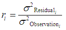
The redundancy number of an observation quantifies the contribution that an observation makes to the total degrees of freedom and is a measure of how close the variance of the residual is to the variance of the observation. The range of possible values is from 0 to 1.
The average redundancy number is a good measure of observational precision and the overall network strength, and the higher the number, the more easily any gross errors will be detected. The redundancy number r for observation i is given by:
|
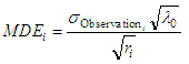
A marginally detectable error identifies the smallest possible magnitude of an outlier that may still be detected at the a and b probability levels; errors of smaller magnitude may not be detected but may adversely affect the adjustment. The MDE is given by:
|
 is determined for the critical values for the a (99%;
double-ended) and b (80%; single-ended) probability levels from
Normal or Fischer distribution tables, eg
is determined for the critical values for the a (99%;
double-ended) and b (80%; single-ended) probability levels from
Normal or Fischer distribution tables, eg
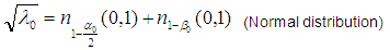
|
Redundancy numbers and marginally detectable errors (MDE) are listed in the summary.
SP1 class testing
|
SP1 definition of Class |
|
Class is assigned to a survey according to the results of a minimally-constrained least squares adjustment which first satisfies the outlier and chi-squared unit variance tests as outlines above. The class for a horizontal adjustment is determined by examining the semi-major axis of each relative error ellipse at the standard (39%, one-sigma) confidence level, to establish if it is less than or equal to the length of the maximum allowable semi-major axis for a particular class level. The class for a vertical adjustment is determined by examination of the standard deviation of each observation at the one-sigma confidence level and comparison with the scale of classes. The following formulae are used to establish the class achieved:
Horizontal control surveys (2D) and vertical control surveys using trigonometric or GPS heighting (1D) :
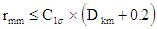
|
Vertical control surveys using differential levelling (1D) :
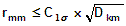
|
 = length of semi-major axis in millimetres
(horizontal), or standard deviation of the observation
(vertical)
= length of semi-major axis in millimetres
(horizontal), or standard deviation of the observation
(vertical) = an empirically-derived factor represented by
historically accepted precision for a particular standard of survey
at the 1-sigma confidence level
= an empirically-derived factor represented by
historically accepted precision for a particular standard of survey
at the 1-sigma confidence level = distance between stations in kilometres.
Values for the factor  are as follows :
| Class | |||||||||||||
| 3A | 2A | A | B | C | D | E | L2A | LA | LB | LC | LD | LE | |
| 1D Trig.Ht/GPS, 2D & 3D horizontal |
1 | 3 | 7.5 | 15 | 30 | 50 | 100 | - | - | - | - | - | - |
| 1D Differential Levelling |
- | - | - | - | - | - | - | 2 | 4 | 8 | 12 | 16 | 36 |
SP1 class testing requires either that the Chi-squared test passes or, if it fails and providing that there were no outliers detected, that the error ellipses are scaled by the a-posteriori sample standard deviation (see under Global chi-squared unit variance test above). If the Chi-squared test fails and the weight matrix is not re-scaled and error ellipses are not scaled, then the reported SP1 classes will not be correct. The safest method is to continue to modify observation standard deviations by trial and error and repeating the adjustment until the Chi-squared test passes.
| Converted from CHM to HTML with chm2web Standard 2.85 (unicode) |